Photo by Markus Spiske on Unsplash
In the previous article, we learned the theoretical concepts of Generative Adversarial Networks.
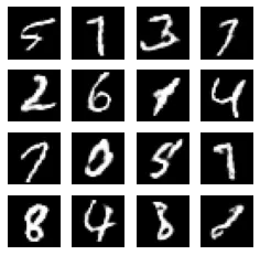
In this article, we’ll understand how to implement Generative Adversarial Networks in Tensorflow 2.0 using the MNIST dataset of digits. Our model should be able to accurately create images similar to MNIST dataset images. Image from MNIST dataset looks like this:

Prerequisites
Before moving ahead please make sure you are updated with the following requirements:
- Basic understanding of Tensorflow 2.0
- Basic understanding of GANs
- Tensorflow 2.0 library with Python 3.6
Let’s jump into code directly
For implementing the network, we need to follow the following steps.
Step 1: Import Libraries
We will need to import these libraries.
1import tensorflow as tf
2import matplotlib.pyplot as plt
3import numpy as np
4import os
5from tensorflow.keras import layers
6import time
7
8from IPython import display
Step 2: Load and Prepare data
1(train_images, train_labels), (test_images, test_labels) = tf.keras.datasets.mnist.load_data()
2train_images = train_images.reshape(train_images.shape[0], 28, 28, 1).astype('float32')
3train_images = (train_images - 127.5) / 127.5
4train_dataset = tf.data.Dataset.from_tensor_slices(train_images).shuffle(60000).batch(256)
In this piece of code, we imported data and reshaped it. Images are represented in the values between 0 to 255. So these image vectors are converted into values between [-1, 1]. Then these vectors are shuffled and converted to batches of 256 images.
Step 3: Create Models
The generator model will take vector of 100 pixels as input and convert that vector into an image of 26 * 26 using the Conv2DTranspose layer. As we are using convolutions, this model will be a DCGAN i.e. Deep Convolutional Generative Adversarial Network.
BatchNormalization layer is used for normalizing the generated image to reduce noise that image. The activation function of “ReLU” is added as another layer in the model.
1def create_generator():
2    model = tf.keras.Sequential()
3
4    # creating Dense layer with units 7*7*256(batch_size) and input_shape of (100,)
5    model.add(layers.Dense(7*7*256, use_bias=False, input_shape=(100,)))
6    model.add(layers.BatchNormalization())
7    model.add(layers.LeakyReLU())
8
9    model.add(layers.Reshape((7, 7, 256)))
10
11    model.add(layers.Conv2DTranspose(128, (5, 5), strides=(1, 1), padding='same', use_bias=False))
12    model.add(layers.BatchNormalization())
13    model.add(layers.LeakyReLU())
14
15    model.add(layers.Conv2DTranspose(64, (5, 5), strides=(2, 2), padding='same', use_bias=False))
16    model.add(layers.BatchNormalization())
17    model.add(layers.LeakyReLU())
18
19    model.add(layers.Conv2DTranspose(1, (5, 5), strides=(2, 2), padding='same', use_bias=False, activation='tanh'))
20
21    return model
Discriminator will do the exact opposite of a generator and convert image into scalar probabilities of whether the image is fake or real. It will use the Conv2D layer for this purpose. Along with the convolutional layer, it will have layer of an activation function “ReLU” and the Dropout layer.
1def create_discriminator():
2    model = tf.keras.Sequential()
3    model.add(layers.Conv2D(64, (5, 5), strides=(2, 2), padding='same', input_shape=[28, 28, 1]))
4    model.add(layers.LeakyReLU())
5    model.add(layers.Dropout(0.3))
6
7    model.add(layers.Conv2D(128, (5, 5), strides=(2, 2), padding='same'))
8    model.add(layers.LeakyReLU())
9    model.add(layers.Dropout(0.3))
10
11    model.add(layers.Flatten())
12    model.add(layers.Dense(1))
13
14    return model
After both the models are created, we’ll move to the next steps.
Step 4: Define Loss and Optimizers
Here, we’re using BinaryCrossentropy from tf.keras.losses API. Using this cross_entropy loss, we’ll make loss functions for discriminator and generator.
1cross_entropy = tf.keras.losses.BinaryCrossentropy(from_logits=True)
2
3def D_loss(real_output, fake_output):
4    real_loss = cross_entropy(tf.ones_like(real_output), real_output)
5    fake_loss = cross_entropy(tf.zeros_like(fake_output), fake_output)
6    total_loss = real_loss + fake_loss
7    return total_loss
8
9def G_loss(fake_output):
10    return cross_entropy(tf.ones_like(fake_output), fake_output)
Now, we’ll create optimizers for generator and discriminator using Adam optimizer from tf.keras.optimizers API with a learning rate of 1e-4.
1generator_optimizer = tf.keras.optimizers.Adam(1e-4)
2discriminator_optimizer = tf.keras.optimizers.Adam(1e-4)
Step 5: Define Training functions
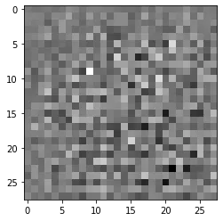
Initially, the generator will generate an image with only random pixels and as time passes, it will make images that are almost similar to the training images. Image from the generator before training looks like the following:
1noise_dim = 100
2num_of_generated_examples = 16
3
4seed = tf.random.normal([num_of_generated_examples, noise_dim])
First, we need to create noise data for passing into the generator model. Then create a function to learn through iterations using the concept of Eager Execution. Please refer to this video for understanding what is Eager Execution as it is out of scope for this tutorial.
1generator = create_generator()
2discriminator = create_discriminator()
3
4@tf.function
5def train_step(images):
6    noise = tf.random.normal([BATCH_SIZE, noise_dim])
7
8    with tf.GradientTape() as gen_tape, tf.GradientTape() as disc_tape:
9      generated_images = generator(noise, training=True)
10
11      real_output = discriminator(images, training=True)
12      fake_output = discriminator(generated_images, training=True)
13
14      gen_loss = G_loss(fake_output)
15      disc_loss = D_loss(real_output, fake_output)
16
17    gradients_of_generator = gen_tape.gradient(gen_loss, generator.trainable_variables)
18    gradients_of_discriminator = disc_tape.gradient(disc_loss, discriminator.trainable_variables)
19
20    generator_optimizer.apply_gradients(zip(gradients_of_generator, generator.trainable_variables))
21    discriminator_optimizer.apply_gradients(zip(gradients_of_discriminator, discriminator.trainable_variables))
GradientTape above is used for creating gradients as we go further and these gradients are applied to optimizers for decreasing the loss function.
1def train_GAN(dataset, epochs):
2  for epoch in range(epochs):
3    start = time.time()
4
5    for image_batch in dataset:
6      train_step(image_batch)
7
8     print ('Time for epoch {} is {} sec'.format(epoch + 1, time.time()-start))
This is the final function to call the train_step function for each batch in the dataset.
Finally, we’ll call our train_GAN function to start training on the image dataset with 500 epochs.
1train_GAN(train_dataset, 500)After going through all the epochs, the generated image looks like this:
Seeing the results
Let’s look at the results in the form of GIF.

It could be seen how our neural networks learn to write integers like a child. We can use the same algorithm for multiple image generators because we only need to change the training images and train again.
What’s next?
GANs could be used for many more domains other than images with the same concept of Generator and Discriminator. Also, read - Contrasting Model-Based and Model-Free Approaches in Reinforcement Learning.


Authors